Replicating “Progress measures for grokking via mechanistic interpretability”
TL;DR
- I replicated the main-text claims of Nanda et al. (2023) with my own code, on four seeds plus the paper’s own weights.
- On the paper’s weights, for 6 of the 9 claims where the paper reports a number, I get their exact results. The three which don’t are the logit approximation as a sum of cosines, the neuron replacement and restriction, and the directions.
- 3 of the 13 claims the paper makes fail on different seeds:
- The MLP computes for every key frequency: not for frequency 5 in seed 3.
- Restricting the neurons to those terms improves the loss: in seed 3 it makes it ~15x worse.
- Memorisation ends before the circuit forms: in seeds 1 and 2, the two phases overlap.
- I found the paper’s unexplained sixth frequency, 31, is a second harmonic of 41, and it cancels a by-product of squaring. These frequencies matter – removing them raises loss by up to 3,200x, but they don’t change accuracy (these frequencies are already known in models without learned attention – see Zhong et al. and Yip et al.)
- The code is hosted on my GitHub (will be public soon).
Setup
Training details
Same as paper
- Task: , with input
a b =. The=sign is token 113, so the vocabulary has 114 tokens. ordered pairs, 30% for training, remainder on test. - Model: 1 layer, , 4 heads of size 32, 512 MLP neurons, ReLU, learned positional embeddings, no LayerNorm, separate embedding and unembedding matrices. Only the MLP has biases.
- Optimiser: full-batch AdamW, learning rate , weight decay 1.0, 40,000 epochs.
- Loss: cross-entropy on the
=position over all 114 logits, computed in float64.
Not stated in paper
- Initialisation: as in the ARENA notebook, weights , , biases zero.
- AdamW betas .
- Learning-rate warmup over the first 10 steps, starting at , then constant with no decay.
- Weight decay applies to every parameter.
- Causal attention mask, with attention scores scaled by . Weights are stored in float32.
- Fourier basis is orthonormal.
- Seeds 0-3 are used, and each seed sets the split and the initialisation.
- Checkpoints every 100 epochs.
- Ablation losses are over all inputs, and the other losses are test-set unless noted.
Reference weights
I run my code on seeds 0-3 for each claim, and figures are produced on seed 0 unless specified otherwise. I use checkpoint weights from Callum McDougall’s Hugging Face repo to compare my code against. These weights appear to be the exact same ones used in the paper – my code reproduces these exactly:
- the paper’s key frequencies (§4.1, p. 4, Fig. 3)
- head 0 at k = 35 and neuron 0 at k = 42 (§4.1, pp. 4–5, Fig. 4)
- 433 well-fit neurons (§4.3, p. 6, Fig. 5)
- the 2.41e-07 baseline (§4.4, p. 7)
- the 0.55% residual (§4.2, p. 6, Fig. 3)
- the Table 1 FVE range (§4.2, p. 6, Table 1)
- −70% at 7.24e-08 for the logit ablation (§4.4, p. 7, Fig. 6)
Scope
- I replicate the main-text claims: grokking (§3), the Fourier multiplication algorithm (§4.1-4.4), and the progress measures and phases (§5). I don’t replicate claims in the appendix or §5.3.
- Runs: four seeds and the paper’s weights.
- Methods follow the paper unless noted.
- The position of key frequencies varies across seeds. My runs learned 4-5 key frequencies, with each seed landing on a different set. So throughout I will compare structure (no. of key frequencies, how much of the Fourier spectrum they account for, and whether individual heads and neurons are dominated by a single one) rather than specific frequencies.
Results
Grokking and its timing (§3)
Claim. Small transformers trained on this task consistently grok, where test accuracy increases sharply, long after achieving perfect train accuracy (§3, p. 3; Fig. 2)
Method. Grokking epoch is the first epoch where the test accuracy >= 99% (as in Phase Boundaries). Final test loss is the loss on the test set at epoch 39,900.
Result.
| Run | Grokking epoch | Final test loss |
|---|---|---|
| Paper (reported) | ~10,000 | — |
| Paper’s weights | 10,600 | |
| seed 0 | 10,800 | |
| seed 1 | 3,800 | |
| seed 2 | 8,500 | |
| seed 3 | 9,700 |
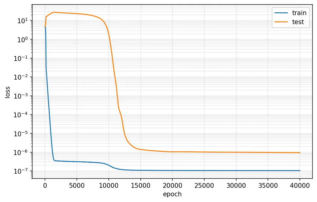
All runs grok. Train loss levels off by at most epoch 1,400 in every run, while test loss stays high until the grokking epoch, which ranges from 3,800-10,800. Final test losses range from to .
Verdict: replicated. All runs grok, and the paper’s run groks at the epoch the paper reports. Timing varies widely between seeds.
Periodicity (§4.1)
Embeddings are sparse in the Fourier basis
Claim. is sparse in the Fourier basis. The paper finds only six frequencies with non-negligible norm. Five of them are key frequencies the rest of the model uses (§4.1, p. 4, Fig. 3).
Method. Same as the paper, except key frequencies were determined as those which raised the loss at least 125x, and non-key frequencies raised the loss at most 1.09x.
Result.
| Run | Key frequencies | Key frequencies’ share of ’s squared norm | Other large frequencies* |
|---|---|---|---|
| Paper (reported) | 14, 35, 41, 42, 52 | — | one, unnamed (p. 4) |
| Paper’s weights | 14, 35, 41, 42, 52 | 93.91% | 31 ≡ 2×41 |
| seed 0 | 1, 5, 31, 42, 53 | 92.26% | 2 = 2×1, 7 ≡ 2×53 |
| seed 1 | 1, 16, 25, 30 | 92.49% | 2 = 2×1 |
| seed 2 | 19, 35, 40, 53 | 95.83% | 38 = 2×19 |
| seed 3 | 5, 10, 19, 41, 48 | 98.78% | none |
*Non-key frequencies with a bar above 1 in the Figure 3 plot. Outside these, the largest bar in any run is 0.73; the weakest key frequency’s bar is 2.48.
Key frequencies of each run, their share of , and other large non-key frequencies.
All four seeds have 4-5 key frequencies at different positions in each seed, which hold 92.3-98.8% of ’s squared norm. The other large frequencies are generally a second harmonic of a key frequency. I find a similar result on the paper’s weights: the sixth frequency in is 31 on its weights, the second harmonic of 41. This is the sixth frequency (k=31) the paper reports but doesn’t name (p. 4). See second harmonics for more on this.
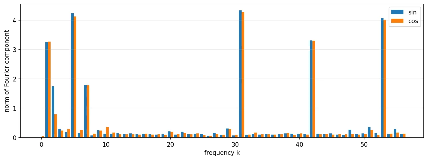
Verdict: replicated. In every run is sparse in the Fourier basis. Every run has the same structure as the paper, where there are 4-5 key frequencies and up to two second harmonics.
Periodicity in the attention heads and MLP activations
Claim. There is a periodic structure in the attention heads and MLP neuron activations at the key frequencies. The logits, written in the 2D Fourier basis over , are significant only at the four product terms of each key frequency , , and (§4.1, p. 4-5, fig. 4).
Method. For head 0 and neuron 0, I report the dominant frequency and its share of the norm. For the logits, each key frequency contributes 4 product cells, so with key frequencies I measure how many of the strongest cells are key cells, and the ratio of the weakest key cell to the strongest non-key cell
Result.
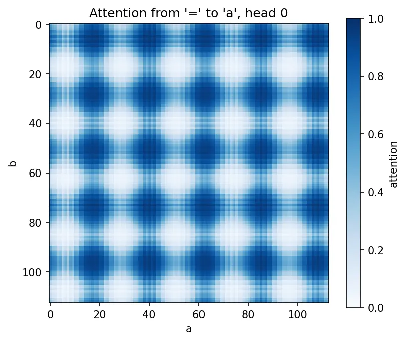
= token to the a token for one input pair, on seed 0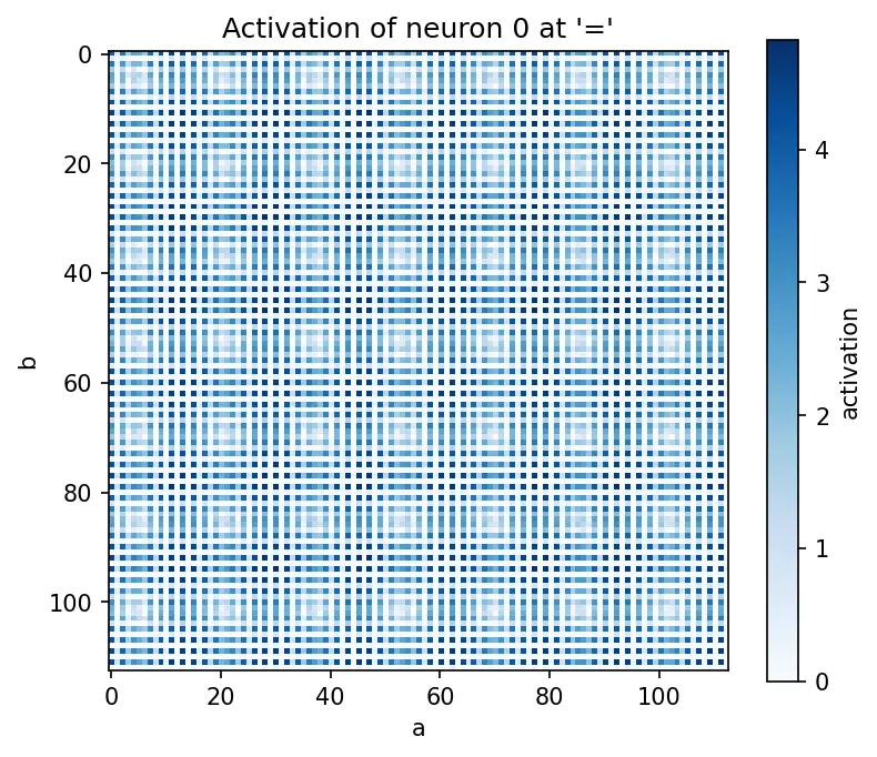
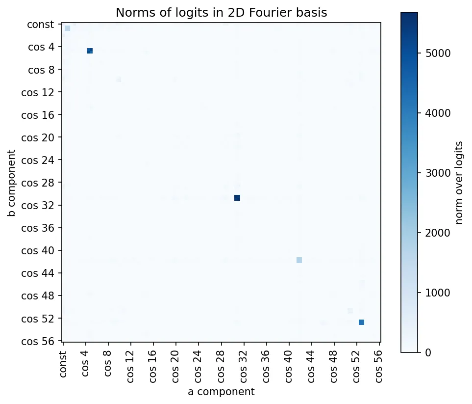
In every run, a single key frequency has the largest share of head 0 and neuron 0, and the key cells hold 96.9-99.0% of the logits’ squared norm. In only seed 3 a key cell falls outside the top , and only just: (sin 20, sin 20) is about 4% stronger than its weakest key cell. In every run the strongest non-key cell is a second harmonic of a key frequency.
| Run | Head 0 | Neuron 0 | Key cells in the top 4n | Weakest key cell ÷ strongest other | Strongest other cell |
|---|---|---|---|---|---|
| Paper’s weights | 35 (97%) | 42 (98%) | 20/20 | 3.91× | (sin 29, const), 29 = 2×42 |
| seed 0 | 5 (95%) | 53 (99%) | 20/20 | 3.48× | (cos 2, const), 2 = 2×1 |
| seed 1 | 25 (87%) | 16 (98%) | 16/16 | 7.12× | (sin 32, sin 32), 32 = 2×16 |
| seed 2 | 40 (99%) | 40 (55%) | 16/16 | 5.29× | (sin 43, sin 43), 43 = 2×35 |
| seed 3 | 10 (95%) | 5 (78%) | 19/20 | 0.96× | (sin 20, sin 20), 20 = 2×10 |
Verdict: replicated. My code on the paper’s weights finds head 0 at and neuron 0 at , which are exactly the paper’s, implying my code finds these frequencies correctly; these frequencies have very high coverage according to the table. As for the periodicity in the logits, for the majority of the seeds, all key cells have significant norm as in the paper. Seed 3 has one key cell missing from the top 4n. The non-key cell is , a second harmonic of the key cell k=10. The key cell which is missing is from frequency 5.
The mechanism (§4.2)
The neuron-logit map uses only the key frequencies
Claim. The neuron-logit map is well approximated using only the key frequencies (§4.2, pp. 5–6; Fig. 3 right):
The sum runs over the key frequencies, and . The vectors have -th entries and , where is the output logit, and are vectors over neurons. With key frequencies this is a rank- matrix (rank 10 for the paper’s five), so the neurons write almost only into directions in logit space. The paper reports a residual under 0.55% (p. 6).
Method. As in the paper, except that I measure the residual as a ratio of squared Frobenius norms. On the paper’s weights this gives exactly 0.55%, so I take it to be what the paper measured (see deviation summary).
Result. The residual contains only 0.20–1.44% of the squared norm of from my weights, so the 2n Fourier directions capture 98.56–99.80% of it.
| Run | Key frequencies | Share of ’s squared norm | Extra in |
|---|---|---|---|
| Paper (reported) | 14, 35, 41, 42, 52 | > 99.45% | — |
| Paper’s weights | 14, 35, 41, 42, 52 | 99.45% | none |
| seed 0 | 1, 5, 31, 42, 53 | 99.63% | none |
| seed 1 | 1, 16, 25, 30 | 99.79% | none |
| seed 2 | 19, 35, 40, 53 | 99.80% | none |
| seed 3 | 5, 10, 19, 41, 48 | 98.56% | 15 = 5 + 10 |
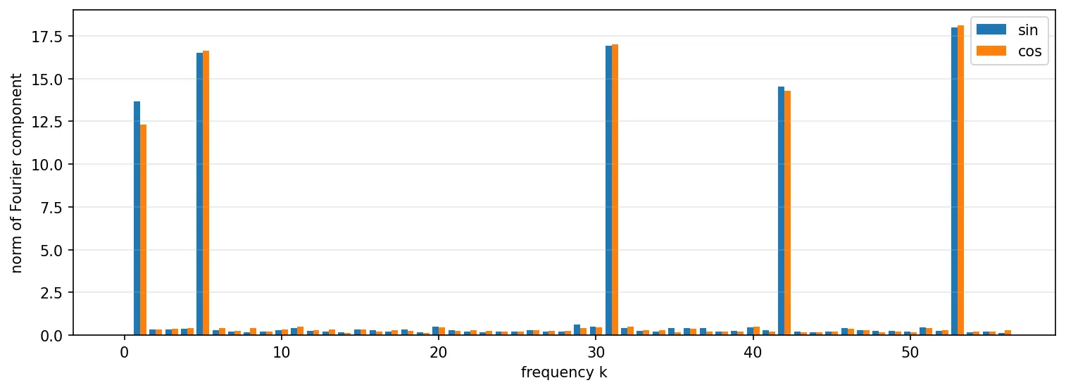
Across all runs, the key frequencies hold 98.56–99.80% of ’s squared norm. ’s large components (plus 15 = 5 + 10 in seed 3) are the run’s key frequencies.
Verdict: replicated My code reproduces the 0.55% residual on the paper’s weights exactly, and my seeds give 0.20-1.44%.
Along the key directions, the neurons compute and
Claim. For each key frequency, the MLP neurons compute and , and reads off those values and multiplies them by and into the logits (§4.2, p. 6; table 1).
Result.
| Run | Directions | Minimum FVE | Median FVE | Fraction above 90% |
|---|---|---|---|---|
| Paper (reported) | 10 | 93.2% | 96.7% | 10/10 (100%) |
| Paper’s weights | 10 | 93.2% | 96.7% | 10/10 (100%) |
| Seeds 0-3 (pooled) | 36 | 19.6% | 97.2% | 31/36 (86.1%) |
| Component | Fourier components of or | FVE |
|---|---|---|
| 84.4% | ||
| 90.5% | ||
| 98.1% | ||
| 98.7% | ||
| 98.1% | ||
| 97.7% | ||
| 87.7% | ||
| 86.8% | ||
| 97.6% | ||
| 97.7% |
Verdict: replicated, except in seed 3. Most directions match the paper – the weak frequencies come out lower. A different result to the paper is in seed 3, where the MLP’s output along the two directions isn’t well described by and , since their FVE is only 19.6% and 34.0%. This matches having no well-fit neurons in seed 3.
Logits as a sum of cosines
Claim. The logits are well approximated by a weighted sum of cosines over the model’s key frequencies, t\sum_k \alpha_k \cos\big(w_k(a+b-c)\big)$. This explains almost all the variance in the original logits (§4.2, p. 6).
Result.
| Run | Key frequencies | Variance explained |
|---|---|---|
| Paper (reported) | 14, 35, 41, 42, 52 | 95% |
| Paper’s weights | 14, 35, 41, 42, 52 | 96.14% |
| seed 0 | 1, 5, 31, 42, 53 | 97.00% |
| seed 1 | 1, 16, 25, 30 | 98.00% |
| seed 2 | 19, 35, 40, 53 | 98.04% |
| seed 3 | 5, 10, 19, 41, 48 | 98.21% |
Verdict: replicated with deviation. There is a small gap between the paper’s number (95%) and my code on its weights (96.14%). I couldn’t figure out why.
Neurons (§4.3)
MLP neuron approximations
Claim. Most neurons (433/512) are well-approximated by degree 2 polynomials of a single frequency (§4.3, p. 6).
Result.
| Run | Key frequencies | Well-fit neurons per | Neurons with over 85% FVE (of 512) |
|---|---|---|---|
| seed 0 | 1, 5, 31, 42, 53 | 93, 54, 99, 40, 105 | 391 (76.4%) |
| seed 1 | 1, 16, 25, 30 | 105, 110, 116, 126 | 457 (89.3%) |
| seed 2 | 19, 35, 40, 53 | 96, 148, 52, 57 | 353 (68.9%) |
| seed 3 | 5, 10, 19, 41, 48 | 0, 114, 41, 91, 58 | 304 (59.4%) |
| Paper’s weights | 14, 35, 41, 42, 52 | 44, 93, 145, 87, 64 | 433 (84.6%) |
In seed 3, key frequency 5 has no well-fit neurons.
Verdict: replicated. I get the exact same results on the paper’s weights as their reported figure. Though the number of neurons which have their variance explained with a single frequency varies much more than the paper’s single figure suggests. For example, the lowest % of neurons with over 85% FVE is 59.4%.
Each neuron writes only its own frequency
Claim. A neuron which has frequency only writes and waves into the logits (§4.3, p.7, fig. 5 right).
Result.
| Run | Well-fit neurons | Median share | Minimum share (cluster) |
|---|---|---|---|
| Seed 0 | 391 | 98.9% | 87.0% () |
| Seed 1 | 457 | 99.6% | 76.0% () |
| Seed 2 | 353 | 99.4% | 78.8% () |
| Seed 3 | 304 | 98.5% | 79.7% () |
| Paper’s weights | 433 | 99.1% | 93.8% () |
Verdict: replicated. In every run, a well-fit neuron’s column lies almost entirely in its own frequency: the median share is 98.5-99.6%, and 99.1% on the paper’s weights. The variance is large though, with each run’s minimum between 76% and 94%.
Ablations (§4.4)
MLP neuron ablations
Claim. Replacing the neurons that were well-approximated by a degree-2 polynomial (identified in MLP neuron approximations) barely increases loss. Restricting each neuron to only its and terms improves the loss (§4.4, p. 7).
Result.
| Run | Neurons replaced | Full-grid loss | Loss after replacing | Change | Accuracy after |
|---|---|---|---|---|---|
| Paper (reported) | 433 | +3% | unchanged | ||
| Paper’s weights | 433 | −37% | 100% | ||
| seed 0 | 391 | −65% | 100% | ||
| seed 1 | 457 | −6% | 100% | ||
| seed 2 | 353 | +52% | 100% | ||
| seed 3 | 304 | +175% | 100% |
| Run | Full-grid loss | Restricted loss | Change |
|---|---|---|---|
| Paper (reported) | −77% | ||
| Paper’s weights | −64% | ||
| seed 0 | −86% | ||
| seed 1 | −22% | ||
| seed 2 | −24% | ||
| seed 3 | +1388% |
- After replacement, in every run, accuracy stays at 100% and losses stay between 1.5e-7 and 1.4e-6, far from the increase from ablating a key frequency.
- The sign and magnitude of change varies between seeds. On the paper’s weights, replacing the same 433 neurons and using the same baseline, my replacement gets -37% while the paper reports +3%. So the replacement step differs in some way I can’t identify.
Verdict: replicated with deviation, except restriction in seed 3. I get a different change in loss after neuron replacement on the paper’s weights versus the paper, but accuracy is still 100%. Restriction improves loss on the paper’s weights and in three of my seeds, but I get a 64% decrease on their weights versus the paper’s reported 77% decrease. On seed 3, restriction increases loss by 1388%. I don’t know why.
Ablating components of the final logits in the Fourier space
Claim. Ablating any key frequency raises the loss sharply, ablating any other frequency barely changes it, and ablating all the non-key frequencies improves it (§4.4, p. 7, Fig. 6).
Result.
| Run | Baseline loss | Removing a key frequency | Removing any other frequency | Keeping only the key frequencies |
|---|---|---|---|---|
| Paper (reported) | large increase (Fig. 6 only) | “does not hurt the model at all” | −70% () | |
| Paper’s weights | 4,300× () to 315,000× () | 0.85× to 1.09× | −70% () | |
| seed 0 | 590× () to 115,000× () | 0.54× to 1.03× | −90% () | |
| seed 1 | 125,000× () to 770,000× () | 0.87× to 1.04× | −45% () | |
| seed 2 | 30,000× () to 2,900,000× () | 0.89× to 1.02× | −52% () | |
| seed 3 | 125× () to 2,100,000× () | 0.82× to 1.01× | −43% () |
Verdict: replicated. I get the same results as the paper on their weights, and the results track with the claim.
directions
Claim. depends on the directions corresponding to the cosine and sine of key frequencies (§4.4, p. 8)
Result.
| Run | Directions | Full-grid loss | Loss onto directions | Change | Accuracy (directions) | Loss onto nullspace | Accuracy (nullspace) |
|---|---|---|---|---|---|---|---|
| seed 0 | 10 | +13.2% | 100% | 4.17 | 10.1% | ||
| seed 1 | 8 | +1.4% | 100% | 4.23 | 12.8% | ||
| seed 2 | 8 | +0.2% | 100% | 4.26 | 11.2% | ||
| seed 3 | 10 (effectively 9)* | −6.2% | 100% | 4.60 | 10.4% | ||
| Paper’s weights | 10 | −0.3% | 100% | 3.98 | 13.7% | ||
| Paper (reported) | 10 | −50% | not stated | 5.27 | not stated |
* ’s and rows are almost parallel
How restricting to the key-frequency directions affects loss
On seed 0, keeping only the 10 directions leaves the loss similar to baseline (). Removing them pushes the loss to 4.17, which is close to uniform (4.73), and accuracy to 10-14%. The paper reports a loss of 5.27, which is much worse than my figure.
Verdict: replicated with deviation. The paper’s numbers don’t reproduce on my code. I get 3.98 loss on the paper’s weights; the paper gets 5.27. Keeping only the 10 directions gives -0.3%, while the paper reports -50%.
Progress measures and phases (§5)
Phase boundaries
Claim. Training is split into memorisation (0-1.4k), circuit formation (1.4k-9.4k) and cleanup (9.4k-14k), and restricted loss improves before test loss does (§5.2, p. 9).
Method. The paper draws its boundaries by eye; I measured them using explicit rules for each:
- End of memorisation – when train loss levels off, defined as the first epoch from which train loss falls by less than 25% over the following 500 epochs. The boundary is not sensitive to the 25%/500 epoch values. Any threshold from 16% to 31%, or any window from 100 to 800 epochs, gives epoch 1,400 in all five runs.
- End of circuit formation – first epoch after memorisation the test loss drops below (the loss of a uniform guess). At initialisation, test loss starts near then rises far above it during memorisation, so when it’s crossed again, the model must have stopped doing worse than uniform guessing.
- End of cleanup – first epoch test loss is within 2x its value at epoch 39,900.
I also added two rules to measure the model’s progression:
- Restricted-loss lead – the number of epochs between restricted loss and test loss each first dropping below .
- Grokking epoch – defined by a minimum test accuracy of 99%.
I chose rules which reproduce the paper’s boundaries on its own weights, then applied them to my seeds. So my code on their weights matches the paper, because the rules were calibrated on that run.
Result.
| Run | Memorisation ends | Circuit formation ends | Cleanup ends | Grokking epoch (test accuracy >= 99%) | Restricted-loss lead |
|---|---|---|---|---|---|
| Paper (reported) | 1,400 | 9,400 | 14,000 | ~10,000 | – |
| Paper’s weights | 1,400 | 9,400 | 14,300 | 10,600 | 1,345 |
| seed 0 | 1,400 | 9,700 | 13,900 | 10,800 | 1,653 |
| seed 1 | 1,400 | 3,100 | 5,200 | 3,800 | 1,000 |
| seed 2 | 1,400 | 7,400 | 10,600 | 8,500 | 863 |
| seed 3 | 1,400 | 8,500 | 11,900 | 9,700 | 1,437 |
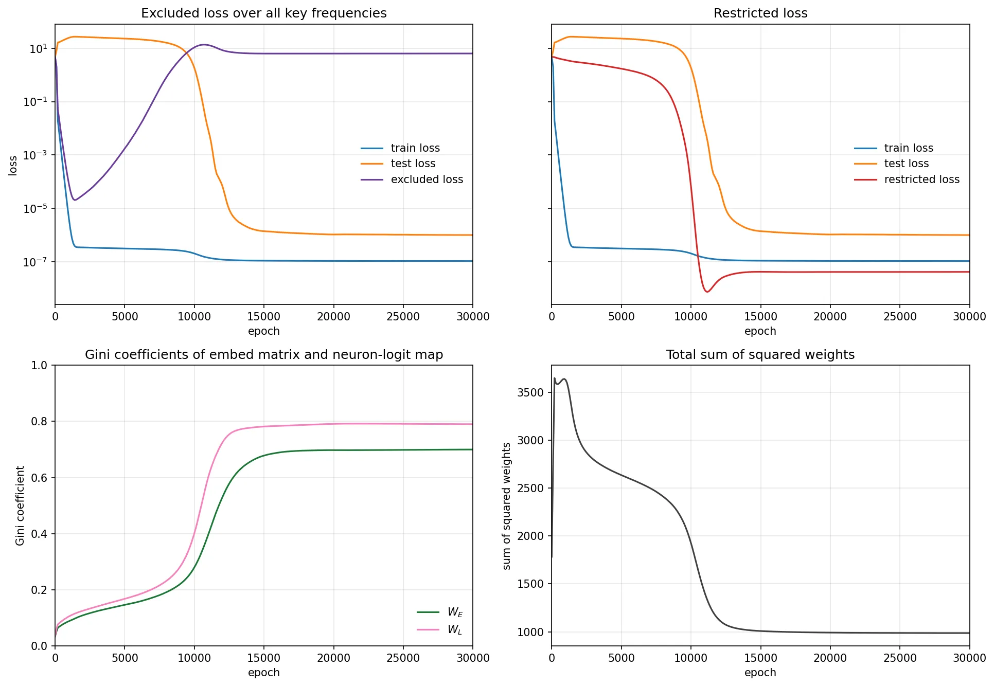
Verdict: replicated. Memorisation ends at epoch 1,400 in every run, because train loss follows the same schedule whatever the seed. Restricted loss is ahead of test loss by 863-1,653 epochs. The length of phases differs with the seed – for example, seed 1 runs through the whole sequence more than twice as fast as any other seed I recorded.
Behaviour within each phase
Claim. Each phase has a characteristic pattern in the progress measures. (§5.2, p. 9).
Method. I tested the number of runs (four seeds plus the paper’s weights) which follow the paper’s claim of the direction of each measure. A loss counts as rising or falling if it changes by more than 10x, a Gini coefficient if it changes by more than 0.1, and the sum of squared weights if it changes by more than 10%. Anything less counts as flat. ’-’ means the paper doesn’t state it.
I leave out train and test loss from the results table because they define the boundaries.
Result.
| Measure | Memorisation | Circuit formation | Cleanup |
|---|---|---|---|
| Excluded loss | ↓ 4/5 | ↑ 5/5 | → 5/5 |
| Restricted loss | → 5/5 | ↓ 5/5 | ↓ 5/5 |
| Gini (, )* | → 3/5 | - | ↑ 5/5 |
| Sum of squared weights | - | ↓ 5/5 | ↓ 5/5 |
*Both and need to match for the Gini row
The three mismatches are in the memorisation phase, for seeds 1 and 2. In these two seeds, circuit formation begins before memorisation ends. Excluded loss reaches its minimum at epoch 900 in seed 1 and 400 in seed 2, against 1,400 in the other runs. In seed 1 there is only a short overlap – excluded loss still falls 164x during memorisation, but ’s Gini coefficient rises by 0.12, just over the 0.1 cutoff. In seed 2 the overlap is larger: excluded loss falls only 3.4x, and ’s Gini rises by 0.13. Seed 2’s excluded loss also only just counts as rising during circuit formation (10.3x, against 253x or more in the other runs).
Verdict: replicated, except in seeds 1 and 2. 8 of the 10 predicted cells match in all five runs. In seeds 1 and 2, the first two phases overlap rather than follow one another.
Second Harmonics
In every run except seed 3, contains components at the second harmonic of a key frequency (). They cancel a by-product the model creates when it squares its key-frequency waves. Secondary-frequency components have been described before in models without learned attention (Zhong et al. 2023; Yip et al. 2024). I find them in the paper’s own model, which has learned attention, and measure how they work there.
Prior work
Nanda & Lieberum (2022) list the paper’s embedding frequencies as 14, 31, 35, 41, 42 and 52, and note that the neurons don’t use 31, without explaining why. Zhong et al. (2023, §3.4 and Appendix D) found circles at double a key frequency in models without learned attention. They call them “accompanying pizzas” and describe them as helping with inputs the main circle handles badly. Yip et al. (2024) find that in these models, a neuron’s secondary frequency has a phase of about twice its main frequency’s phase plus π. That is the phase that cancels the doubled term produced by squaring the main frequency.
The extra frequencies are doubles of key frequencies
The second harmonic of a key frequency is the frequency . On 113 points, frequencies and give the same wave, since for every integer (the sine just flips sign). So when , the second harmonic appears at . For example, the paper’s weights have key frequency 41, whose second harmonic appears as . In the tables, means they are the same frequency.
| Run | Key frequencies | Extra embedding frequencies | Next-strongest logit frequencies |
|---|---|---|---|
| seed 0 | 1, 5, 31, 42, 53 | , | , , |
| seed 1 | 1, 16, 25, 30 | , , | |
| seed 2 | 19, 35, 40, 53 | , , | |
| seed 3 | 5, 10, 19, 41, 48 | none (but its key 10 is ) | , , |
| Paper’s weights | 14, 35, 41, 42, 52 | , , |
The paper’s unused sixth frequency, 31, is the double of key frequency 41. Seed 3 has no extra frequency – its double of 5 is one of the key frequencies.
Second harmonics matter, mostly on the hardest inputs
The number of frequencies with norm varies with the seed. To check whether these frequencies were just a leftover artifact of memorisation, I plotted the norms of them:
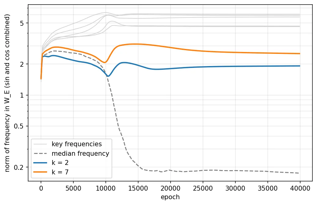
The frequencies don’t decay, so they were likely a part of the solution. During cleanup, the non-key frequencies shrink 2-5x, but the harmonics don’t. Removing them from raises loss 30-3,200x, but test accuracy is still 100%. Hence they only make the model more confident, as opposed to being required to answer correctly.
The harmonics only use the attention heads’ OV circuits. I removed the second harmonics from for one circuit at a time. Removing them from the OV circuit raises seed 0’s test loss 300x (the same as removing them from entirely), while removing them from the QK circuit changes it by less than 1%.
| Seed 0 | Worst input | 1st percentile | Median |
|---|---|---|---|
| nothing removed | 8.94 | 11.79 | 17.15 |
| and removed (doubles) | 2.27 | 5.71 | 15.63 |
| removed (key frequency) | 3.56 | 11.41 |
Removing the harmonics lowers the margin on the worst input from 8.94 to 2.27. Margins are in logits, so a margin of means the model rates the correct answer times more likely than the strongest wrong answer. On that input, the correct answer goes from about 7,600 times more likely than the runner-up to about 10 times. The margin stays positive on every input, so the model still gets every answer right. Removing key frequency 1 instead pushes the worst margin below zero (), so the model gets that input wrong.
Removing the harmonics lowers the margin by 6.67 at the worst input and 6.08 at the 1st percentile, but only 1.52 at the median. On the other hand, removing key frequency 1 lowers the median by 5.74. So key frequencies matter everywhere, while the harmonics matter mostly on the hardest inputs.
Second harmonics cancel a by-product of squaring
They cancel a side effect of how the network multiplies waves. To add and , the neurons for frequency effectively square waves, and squaring a wave produces a wave at double the frequency . This results in part of each neuron’s activation varying at as changes. Those neurons write their output as a frequency- pattern over answer , so that part comes out as a pattern peaking at = , and likewise = . So, squaring a frequency- wave creates a by-product in the logits:
and are its fitted strength and phase.
It peaks at and instead of at the answer . This single term accounts for 71–100% of the margin each by-product costs:
| Run | By-product in the logits | Double in ? | Margin cost (whole) | Margin cost: (/ term) | Share |
|---|---|---|---|---|---|
| seed 0 | yes | 1.47 | 1.05 | 71% | |
| seed 0 | no | 1.40 | 1.40 | 100% | |
| seed 0 | yes | 0.12 | 0.12 | 100% | |
| seed 1 | yes | 0.43 | 0.41 | 95% | |
| seed 2 | yes | 0.53 | 0.51 | 96% | |
| seed 3 | no | 0.46 | 0.43 | 93% | |
| Paper’s weights | no | 0.44 | 0.43 | 98% | |
| Paper’s weights | yes | 0.27 | 0.23 | 85% | |
| Paper’s weights | no | 0.18 | 0.14 | 78% |
The harmonics in cancel most of this by-product. Removing them makes it 2.4–5.3× larger in the logits (seed 3 has no strong doubles to remove, so nothing changes there). If the by-product is also removed from the logits, the loss decreases: in seed 0, test loss rises from to with the harmonics removed, and falls back to 3.6e-7 with the by-product removed.
The by-product explains seed 0’s high test loss
Seed 0 ends training with the highest test loss of any run (, against for seeds 1 and 2). The by-product explains most of this, since it matters most when it falls near the strongest wrong answer. Removing the by-product improves seed 0’s test loss about 4x, from 9.4e-7 to 2.2e-7.
On the hardest 1% of seed 0’s test inputs, the strongest wrong answer is usually (65% of the time) 47 away from the correct one. The three strong key frequencies (5, 31, and 53) score these two answers almost the same, so the two weakest key frequencies, 1 and 42, supply 77% of the gap between them. These are the frequencies whose by-products cost the most margin: 1.47 and 1.40, against at most 0.53 for any by-product in the other runs.
Limitations
- Five runs with the same setup. The harmonics appear in every run except seed 3.
- Not every by-product gets a double, e.g. seed 0’s by-product at 29, and the paper’s weights’ by-products at 28 and 29 have no matching double in . I don’t know why the model cancels some by-products and not others.
- The fitted term doesn’t explain all of the cost. It accounts for at least 93% in six of the nine cases, but only 71–85% in the other three, and I haven’t identified the rest.
Deviation summary
| Item | Paper | Paper’s weights (my code) | My seeds | Reason |
|---|---|---|---|---|
| Bar heights (Fig. 3) | Tallest bar 2.29 in , 2.22 in | 4.15 in , 16.7 in | 4.33–5.31 in , 18.1–24.2 in | Paper plotting convention. |
| Squared-norm residual | “Frobenius norm that is under 0.55% of the norm of ” (p. 6) | 0.55% of the squared norm (7.4% of the norm) | 0.20–1.44% of the squared norm | Paper’s norm is squared. |
| Neuron replacement | +3%, 433 neurons | −37%, the same 433 neurons | −65% to +175%; 100% accuracy | Unexplained. The baseline () and the 433 neurons match the paper, so the difference is in the replacement step, and the paper’s released notebook doesn’t include this ablation. |
| Restriction to | −77% (to ) | −64% | −86% to −22% (seeds 0–2); +1388% (seed 3), 100% accuracy | Using restricted loss on the paper’s weights gives the −77% as in the paper. But the paper quotes a loss of , while I get , which rounds to . Uncertain what would close the gap, or whether this is a coincidence. |
| Keeping only the directions | −50% | −0.3% | −6.2% to +13.2% | Unknown. |
| Projecting onto the nullspace | 5.27, “worse than uniform” | 3.98 (uniform: ) | 4.17–4.60 | Unknown. |
| Logit fit | 95%; loss to | 96.14%; loss to | 97.00–98.21% | Unknown. |
| Low FVE for weak frequencies | 93.2–98.2%; lowest at | Same; is the weakest key frequency | 5 of 36 below 90%, all at the weakest key frequencies: seed 0’s and ; seed 3’s (down to 19.6%) | Variance left over in seed 0 was due to the by-product (see Second Harmonics). Unsure on seed 3. |
| The paper’s “test loss” being full-grid loss | Calls “test loss” (pp. 6, 16) | Full grid ; test set | Full grid –; test set – | The paper defines test loss on the held-out pairs (p. 3), but the baselines it calls “test loss” (pp. 6, 16) are the loss on all inputs. |
| Phases overlap (seeds 1, 2) | Memorisation ends by ~1,400 in all runs, then train loss stays flat (p. 9; C.2.1, p. 22) | Ends at 1,400; all 10 cells match | Memorisation ends at 1,400 in every seed. Seeds 0 and 3 match all 10 cells. Seeds 1 and 2: excluded loss bottoms out early (900 and 400) and ’s Gini rises during memorisation | The memorisation and circuit formation phases overlap on some seeds. |